In today’s rapidly evolving business landscape, staying ahead of the competition requires more than just a great product or service. It demands a deep understanding of the market, consumer behavior, and emerging trends. This is where the market research process becomes invaluable. In this blog post, we will delve more into market research and explore...
There is never a wrong time to do market research. However, most research projects are birthed because a company or organization is at a crossroads. Whether you’re a startup or Fortune 500 company, you’ll have critical decisions to make. This blog will detail common market research examples and how our clients have used them to...
Conjoint Analysis vs. Discrete Choice Modeling: The Main Differences
Emily Rodgers
The short answer: Conjoint analysis is the broader survey technique where respondents evaluate or rate full product profiles built from multiple attributes. Discrete choice modeling is the choice-based version of that technique, rooted in econometric theory, where respondents pick one option from a small set of competing alternatives, the way they would on a shelf or a website.
Conjoint is the better fit when you’re optimizing product features. Discrete choice is the better fit when you need pricing sensitivity, market share estimates, or competitive simulations.
If you’ve scoped a pricing research study or a new product launch with a research partner, there’s a good chance “conjoint” and “discrete choice” came up in the same conversation, often used almost interchangeably.
That’s not entirely wrong. Discrete choice modeling is technically a type of conjoint analysis. But in practice, the two terms point to different respondent tasks, different statistical engines, and different business decisions.
Mixing them up isn’t just a vocabulary problem. It can mean designing a study that gives you the wrong kind of output for the decision you’re trying to make.
Below, we’ll break down what each method actually measures, when to use one over the other, and how the common variations fit into the decision.
Identify which product features buyers value most with expert-led studies.
Conjoint analysis is a survey-based research method that asks respondents to evaluate products or services built from a combination of attributes and attribute levels.
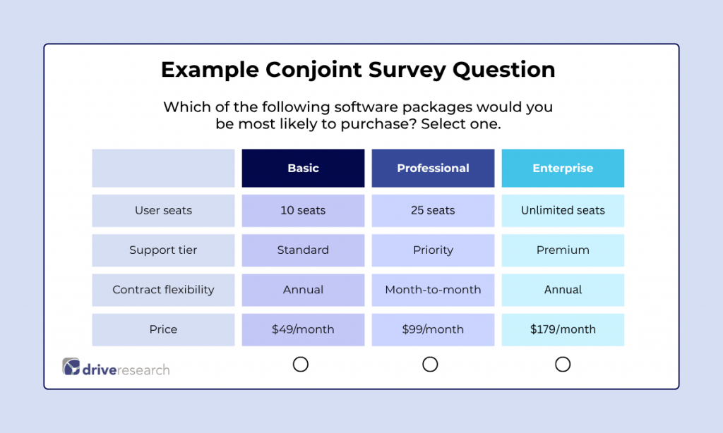
Instead of asking someone to rate price, features, and brand separately, conjoint bundles them into full product profiles and asks respondents to react to the whole package.
A typical setup might define a product across attributes like price, material, warranty length, and color.
Each attribute has several levels (price might range from $50 to $150, warranty from 1 to 5 years). The survey generates dozens of profile combinations, and respondents either rank them, rate them, or choose between a handful at a time.
The output is a set of part-worth utility scores for every attribute level tested.
Those scores tell you how much value respondents place on, say, a 3-year warranty versus a 1-year warranty, independent of every other attribute.
Stack the utilities together and you get a picture of which combination of features and price points respondents value most.
In our experience, conjoint works best when the goal is narrowing down a finite set of design decisions rather than modeling an open-ended market.
What Is Discrete Choice Modeling (DCM)?
Discrete choice modeling is built on Random Utility Theory, the idea that people choose the option that delivers the highest perceived value to them at the moment of decision.
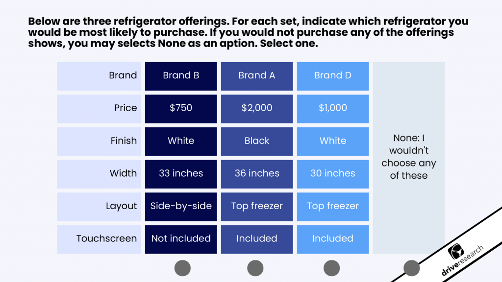
In a DCM study, respondents are shown a set of competing product profiles, often three or four at a time, and asked to pick the one they would actually buy.
Many designs also include a “none of these” option, which matters more than it sounds. Without it, you force a sale that might not happen in real life.
Respondents repeat this exercise across several screens, each time with a different combination of products and attribute levels.
The data is analyzed using multinomial logit or hierarchical Bayes models, which estimate the probability that a given product configuration gets chosen over the alternatives.
The result is something you can plug into a market simulator.
The Key Takeaway: Want to know what happens to your market share if a competitor drops their price by 10%? Or if you add a feature your competitor doesn’t have? DCM is built to answer exactly that kind of question.
Conjoint vs. Discrete Choice: The Core Differences
Here’s how the two methods stack up side by side before we break each factor down:
Factor
Conjoint Analysis
Discrete Choice Modeling
Respondent task
Rate or rank full product profiles, often one at a time
Pick one product from a small competing set, frequently with a “none” option
Statistical model
Regression-based (OLS or hierarchical Bayes) on rating/ranking data
Multinomial logit or HB-MNL, grounded in Random Utility Theory
What it outputs
Part-worth utilities and attribute importance scores
Choice probabilities and market share estimates
Realism
More abstract; respondents evaluate profiles individually
Closer to real-world shopping; competing options shown side by side
Pricing, willingness to pay, market share and competitive simulation
Respondent Task
Conjoint respondents typically rate or rank individual profiles, sometimes one at a time, sometimes in small comparison sets. It asks for more granular feedback on each option individually.
Discrete choice respondents pick a single winner from a set of competing alternatives, often with the option to walk away entirely. The DCM task mirrors a real purchase decision more closely.
Underlying Statistical Model
Traditional conjoint relies on regression-based estimation, frequently ordinary least squares or hierarchical Bayes, to calculate part-worth utilities from rating or ranking data.
Discrete choice modeling is grounded in Random Utility Theory and estimated using multinomial logit or hierarchical Bayes multinomial logit (HB-MNL), which models the probability of choice rather than a preference score. The math is different because the underlying question is different: how much do you like this, versus what would you actually pick.
What Each Method Outputs
Conjoint produces part-worth utilities and attribute importance scores. You’ll know that warranty length matters more to your audience than color, and you’ll know the relative value of each level within warranty length.
Discrete choice modeling produces choice probabilities and, when fed into a simulator, market share estimates. You’re not just learning what people value. You’re estimating how a specific product configuration would perform against named or hypothetical competitors in the market.
Realism and Ecological Validity
This is where the two methods diverge the most in practice.
A discrete choice exercise, especially one with a “none” option, behaves more like a real shopping decision. Respondents see a handful of competing products and either pick one or walk away, the same way they would scan a shelf or compare options online.
Conjoint’s full-profile ratings task is useful for isolating attribute-level preferences, but asking someone to individually rate a dozen or more hypothetical products in a row can start to feel abstract, disconnected from how they’d actually shop.
Stop guessing what drives purchases with custom trade-off research.
If the question is which combination of features to build into a new product, conjoint is usually the right tool. It isolates the value of each attribute level cleanly, which makes it well suited for R&D and product teams deciding what to include in version 2.0.
Concept Testing With Defined Attributes
When you already know the attributes that matter (price tiers, material options, service levels) and need to understand how respondents weigh them against each other, conjoint gives you a defensible, attribute-by-attribute breakdown.
Real world use case:
We used this approach for a healthcare client launching a direct-to-consumer service for IBD patients, pairing conjoint with feature-level willingness to pay to land on a defensible price point and the messaging to support it.
Traditional conjoint performs best with a manageable design, typically 4 to 6 attributes with 2 to 5 levels each. Push past that and respondent fatigue starts contaminating the data. If your attribute list is long, that’s usually a sign to either trim it first (a quick MaxDiff exercise works well here) or move toward a choice-based design built to handle more complexity.
When to Use Discrete Choice Modeling
Pricing and Willingness to Pay
DCM is the stronger choice when price sensitivity is the central question. Because respondents are choosing among competing products at different price points, and can opt out entirely, the resulting model produces a more realistic demand curve than a ratings-based conjoint can.
This is the method we lean on most often when a client’s real question is “how much can we charge.”
If the deliverable needs to feed a market simulator, projecting share of preference for a new product against the current competitive set, DCM is built for it. The choice-based data translates directly into probability estimates that a simulator can use.
Competitive Scenario Testing
DCM also handles “what if” questions well.
What happens to our share if Competitor A launches a lower-priced version?
What if we add a feature they currently have exclusively?
Because the model is estimating choice probability across named alternatives, you can swap attributes in and out of the simulation to test scenarios without fielding a new study every time.
Common Variations of Each Method
Choice-Based Conjoint (CBC)
CBC is the most widely used form of discrete choice modeling in commercial research today. Respondents see sets of competing product profiles and pick their preferred option, often with a “none” choice included. When people say “discrete choice modeling,” they’re frequently describing choice based conjoint specifically.
Adaptive Conjoint Analysis (ACA)
Adaptive conjoint analysis is a legacy method that adjusts which questions a respondent sees based on their previous answers, reducing the burden of evaluating every possible attribute combination.
It’s largely been replaced by CBC and adaptive CBC designs in modern practice, but it’s worth knowing the term if you’re reviewing older research literature or working with a partner who still offers it.
Menu-Based Choice (MBC)
MBC asks respondents to build their own product by selecting add-ons to a base offering, the same way a customer configures a subscription tier or a car trim package. It’s particularly useful in telecom, SaaS, and any category where bundling and add-on pricing drive revenue.
MaxDiff as an Alternative
MaxDiff isn’t a conjoint or discrete choice method at all. It asks respondents to pick the “best” and “worst” item from a set, which produces a clean priority ranking rather than a trade-off model.
We bring it up here because it’s a useful first step before either conjoint or DCM: run MaxDiff to narrow a long attribute list down to the ones that actually matter, then build your conjoint or discrete choice design around that shorter list.
Useful resource: In our blog post MaxDiff vs. Conjoint Analysis, discover which research method fits your next big decision.
How to Choose Between Conjoint and Discrete Choice
Start With the Business Decision
Before picking a method, get specific about what decision the research needs to support.
“Which features should we include” points toward conjoint.
“What should we charge” or “what’s our projected market share” points toward discrete choice modeling.
We’ve had clients come to us asking for a conjoint study when what they actually needed was a pricing simulator, and getting that decision right up front saves both budget and timeline.
Consider Your Attribute List
A short, well-defined attribute list (4 to 6 attributes) works fine with traditional conjoint. A longer list, or one where competitive context matters, usually performs better as a choice-based design, which can handle more complexity without overloading any single respondent.
Factor in Sample Size and Cost
Discrete choice modeling with hierarchical Bayes estimation generally calls for a larger sample, often 300 to 500 respondents per segment, to produce stable individual-level estimates. Traditional conjoint with a tighter attribute set can sometimes run leaner. Cost differences between the two are usually driven more by sample size and analysis complexity than by the survey programming itself.
Plan for the Output You Need
If the end goal is a market simulator your team can use for ongoing “what if” scenarios, that requirement alone often settles the question in favor of discrete choice modeling.
If you just need to know which attribute levels drive preference, without needing to simulate share against named competitors, conjoint’s part-worth output is usually sufficient and less costly to produce.
Another real world example:
We worked with a window and door manufacturer, on a conjoint study to assess how a new double-hung window line would affect their product portfolio and competitor market share.
The study tested how different window attributes were valued by the market, and the results gave our client the confidence to launch the new line, with specific guidance on which regions to prioritize for growth.
Not sure which method fits your project? That’s exactly the kind of question we help clients sort out before a survey gets built.
We’ve run both conjoint and discrete choice studies across building materials, financial services, consumer goods, and healthcare — and the right call has never been the same twice. (I won’t give up my em dashes. I promise this is a real person writing this blog)
If you have a similar decision in front of you, reach out. We’ll help you scope the right design from the start.
We analyze more than data—we also track how our site is used to improve your experience. Cookies help us understand what’s working so we can deliver the most relevant insights. Click “Accept” to enable full functionality.
Functional
Always active
The technical storage or access is strictly necessary for the legitimate purpose of enabling the use of a specific service explicitly requested by the subscriber or user, or for the sole purpose of carrying out the transmission of a communication over an electronic communications network.
Preferences
The technical storage or access is necessary for the legitimate purpose of storing preferences that are not requested by the subscriber or user.
Statistics
The technical storage or access that is used exclusively for statistical purposes.The technical storage or access that is used exclusively for anonymous statistical purposes. Without a subpoena, voluntary compliance on the part of your Internet Service Provider, or additional records from a third party, information stored or retrieved for this purpose alone cannot usually be used to identify you.
Marketing
The technical storage or access is required to create user profiles to send advertising, or to track the user on a website or across several websites for similar marketing purposes.